How are physical and social spaces related?
– cognitive agents
as the necessary “glue”
Bruce
Edmonds
Centre for Policy Modelling,
http://bruce.edmonds.name
Introduction
Even social entities such as: humans, animals, households, firms etc. exist in physical space. The way these entities are distributed in that space is frequently important to us. Some of this distribution can be clearly attributed to economic and environmental factors that are essentially independent of the social interaction between these entities[1]. However it is overwhelmingly likely that some of the distribution is due to the interaction between these entities – i.e. the spatial organisation of the collection of such entities is (at least partially) self-organised via processes of social interaction.
It is difficult to study such self-organisation using purely statistical techniques. Statistical techniques are more suited to dealing with aggregate properties where the deviation from these properties in particular cases can be considered as essentially random. Thus not only can the detail of the spatial organisation be lost in the process of aggregation but in many social cases the distribution of the deviations are not random. Furthermore statistical models, in practice, require fairly drastic assumptions in order to make them amenable to such techniques.
Mathematical models (e.g. those expressed as differential or difference equations) have the potential to capture the self-organisation, but only by disaggregating the model into many separate sets of equations for each entity (or place). This, except in a few special cases where strong assumptions hold, makes any analytic solution impossible. Thus if one tries to apply such techniques to study self-organised distribution one usually ends up by numerically simulating the results, rather than exploiting the analytic nature of the formalism.
It is for these reasons that the study of such self-organisational processes has been advanced primarily through the use of individual-based computational simulations. These are simulations where there are a number of individual entities in the simulation which are named and tracked in the process of the computation. It is now well established that considerable complexity and self-organisation can result in such models even where the properties and behaviour of the individuals in the models are fairly simple. Many of these models situate their component individuals within physical space, so that one can literally see the resulting spatial patterns that result from their interaction (Axtell and Epstein).
Some of these individual-based models seek to capture
aspects of communicative interaction between actors. That is, the interaction between the modelled
entities goes beyond simple cause and effect via their environment (as in
market mechanisms, or the extraction of common resources) but tries to include
the content or effects of meaningful communication between the actors. Another way of saying this is that the actors
are socially embedded (Granovetter,
However, in the modern world humans have developed many media and devices that, in effect, allow communication at a distance[2]. For example, farmer may drive many miles to their favourite pub to swap farming tips rather than converse with their immediate neighbours. Thus the network represented by the communication patterns of the actors may be distinct from the spatial pattern. Recently there have been some models which seek to explore the effects of other communicative topologies. There has been particular focus on “small world” topologies, on the grounds that such topologies have properties that are found among the communicative webs of humans, in particular the structure of hyperlinks on the Internet. However such models are (so far) divorced from any reference to physical space, and focus on the organisation and interactions that can occur purely within the communicative web.
There have been very few models which explicitly include actions and effects within a physical space as well as communication and action within a social space. This paper argues that such models will be necessary if we are to understand how and why human entities organise themselves in physical space. A consequence of such models will involve a move away from relatively simple individual-based simulations towards more complex agent-based simulations due to the necessary encapsulation of the agents who act in space and communicate with peers. Thus some sort of cognitive agency will be necessary to connect the communication with the action of the individuals. This parallels Carley’s call for social network models to be agentified (Carley).
Thus this paper argues that such agency will be unavoidable in adequate models of the spatial distribution of human-related actors and, further, that the spaces within which action and communication occur will have to be, at least somewhat, distinct. Thus the burdon of proof is upon those modellers who omit such aspects.
To establish the potential importance of the interplay between social and physical spaces, and to illustrate the approach I am suggesting, I exhibit a couple of agent-based simulations which involve both physical and social spaces. The first of these is an abstract model whose purpose is simply to show how the topology of the social space can have a direct influence upon spatial self-organisation, and the second is a more descriptive model which aims to show how a suitable agent-based model may inform observation of social phenomena by suggesting questions and issues that need to be investigated.
Example 1 – The Schelling Model of Racial Segregation Extended with a Friendship Network and Fear
The Schelling model of racial segregation
To illustrate the interplay of social and physical spaces, I go back to Schelling’s pioneering model of racial segregation (Schelling 1969). This was a simple model composed of black and white counters on a 2D grid. These counters are randomly distributed on the board to start with (there must be some empty squares left). There is a single important parameter, c, which is the ratio of counters of its own colour among the counters in its immediate neighbourhood (see the first diagram in Figure 1 below) below which the counter will seek to move. Each generation of this game, each counter is considered and if the ratio of same coloured counters in its neighbourhood is less than c then it randomly selects an empty square next to it (if there is one) and moves there.
Figure 1. Neighbourhoods of distances 1, 2 and 3 respectively in the 2D Schelling model
The point of the model was that self-organised segregation of colours resulted for surprisingly low levels of c, due to the movement around the ‘edges’ of segregated clumps. The interpretation is that, even if people are satisfied with their location if only 40% of their neighbours are the same colour as them, then racial segregation could result – it does not take high levels of intolerance to cause such segregation. Figure 2 below shows three stages of a typical run of this model for c=0.5 and a neighbourhood of distance 1.
Figure 2. A typical run of the Schelling model at iterations:0, 4, and 40 (c =0.5)
Figure 3 is a graph of the typical outcomes of this model in terms of the critical parameter, c, and the final average of the proportion of each counter’s neighbours who are of the same colour – this is an indication of the extent of the segregation that occurs. One can see that segregation gradually increases from low levels of c until at c = 0.35 a significant level of self-organised segregation is the result. The maximum is somewhere between c = 0.6 and c = 0.65. Above this level the segregation drops sharply off. This is due to the impossibility of all counters finding positions with 75% like counters and so counters at the edges of segregated clumps are continually randomly relocating destroying any clumping. As discussed in (Edmonds and Hales 2003) this is not a fault of the model since its purpose was to show, as simply as possible, how segregation could occur at low levels of intolerance.
Figure 3. The variation of resulting
segregation with levels of intolerance
(distance-1 neighbourhoods)
It is interesting to note that, even in Schelling’s model the social topology (in this case the neighbours each counter considers in the decision to move or not) can have an effect. Figure 4 shows the corresponding graph to Figure 3 for runs of the Schelling model with a neighbourhood of distance 3. Since each counter has many more neighbours (in the later case 56 of them) it is more likely that one is satisfied with a random mix at the beginning for low values of c. In other words, it is much less likely that a counter will find itself attached to a monolithic clump of the other colour at the beginning and so will not ever move. This “flattening” of segregation for low levels of c (i.e. c < 0.35) depends upon the random initialisation of the model. If one started from an already segregated pattern then increasing the size of neighbourhoods would have a less significant effect.
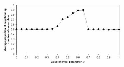
Figure 4. The variation of resulting
segregation with levels of intolerance
(distance-3 neighbourhoods)
The extended model
I have extended this model by adding an explicit “social structure” in the form of a friendship network. That is a directed graph between all counters to indicate who they consider are their friends. The topology of this network is randomly determined at the start according to three parameters: the number of friends, the local bias and the racial bias. The number of friends is how many friends each counter is allocated. The local bias controls how many of a counter’s friends come from the local neighbourhood – a value of 1 means all its friends come from its initial neighbourhood, and a value of 0 means that all counters are equally likely to be a friend. The racial bias controls the extent to which a counter's friends have its own colour – a value of 1 means that all its friends have the same colour as itself and a value of 0 that it is unbiased with respect to colour and friendship. In this model this structure is then fixed for the duration of the run. This network has several functions: firstly, influence only occurs from a counter to a friend, secondly, if it has sufficient friends in its neighbourhood a counter is unlikely to seek to move and, thirdly, (depending on the movement strategy set for the run) if a counter has decided to move it may seek to move nearer to its friends (even if this move is not local).
The motivation for moving is different as well. Instead of being driven by intolerance, the idea is that it is driven by fear. Each counter has a fear level. This is increased by incidents (which occur at random) happening in their location and by fear being transmitted from friend to friend. There are two critical levels of fear: when the fear reaches the first level the counter (randomly with a probability each time) transmits a percentage of its fear to a friend, this transmitted fear is added to the friends fear. Thus fear is not conserved but naturally increases and feeds on itself. When fear reaches the second critical level the counter seeks to move to be closer to move friends (or away from non-friends). It only moves if there is a location with more friends than its present location. When it does so its fear decreases. Fear also naturally decays each iteration to represent a sort of memory effect. This is not a very realistic modelling of fear, since fear is usually fear of something, but it does seem to be cumulative and caused in others by communication. The incidents that cause fear occur completely randomly over all locations with a low probability. The other reason for moving is simply that a counter has no friends in its neighbourhood. However the purpose of this model is simply to demonstrate that social networks can interact with the physical space in ways that significantly affect the outcomes.
Thus in this model the influence of counter colour upon counter movement is indirect: counter colour influences the social structure (depending on the local and racial biases) and the social structure influences relocation. Thus I separate its position in space and the social driving force behind relocation.
The dynamics of this model are roughly as follows. There is some movement at the beginning as counters seek locations with some friends but initially levels of fear are zero. Slowly fear builds up as incidents occur (depending on the rate of forgetting compared to the rate of incidence occurrence). Fear suddenly increases in small “avalanches” when it reaches the first critical level in many counters for fear is suddenly transmitted over the social network causing others to pass the critical level etc. When fear reaches the second critical level then counters start moving towards where its friends are concentrated (or away from non-friends depending on the move strategy that is globally set). This process continues and eventually settles down as counters only move if they can go to where there are more friends than its current location.
Table 1 shows some of the key parameters of the simulation for the range that I will talk about. I have chosen this range of values, because it is relevant to my point and seems to be the critical region of change in this model. The three parameters I will vary are those that affect the topology of the social network: the number of friends each counter has; the bias towards (initially) local friends; and the racial bias. Each of these parameters are tried with each of 5 values, giving 125 runs in total. In each of the graphs below each line represents the average value over 25 different runs.
Table 1. Parameter settings
|
Parameter/setting |
Range of values |
|
Number of Cells Up |
20 |
|
Number of Cells Across |
20 |
|
Number of Black Counters |
150 |
|
Number of White Counters |
150 |
|
Neighbourhood Distance |
2 |
|
Local Bias |
0.45-0.55 |
|
Racial Bias |
0.75-1.0 |
|
Num Friends |
2-10 |
The greatest effect results from the number of friends each counter has, i.e. the connectedness of the social network.
Figure 5. The average of the average fear level for runs with different numbers of friends
Figure 5 shows the average fear levels for runs with different number of friends (25 runs each). The fear levels increase exponentially due to the fact that counters (probibillistically) communicate a proportion of their fear – an interpretation of this could be that if they are more fearful they communicate more fear. The amount of fear increases with the number of friends each counter is allocated up to the value of 8 but this decreases for the runs with 10 friends. There seems to be two different competing effects: the more connected the social network the more fear is communicated and multiplied but also a high number of friends allows counters more opportunities to move and hence to dissipate a chunk of their fear. Figure 6 shows the average number of communications and Figure 7 the average number of movements. It is clear that the more friends one has the more chances there are of moving to a location with a higher number of friends (who themselves might well move etc.) so that the simulation takes a lot longer to “settle down” to a situation where no one can move somewhere better. It is notable that in Figure 6 the number of communications is initially greatest for the runs with 10 friends but then drops down below those runs with 6 or 8 friends.
Figure 6.
The average of the number of communications
for runs with different numbers of friends
Figure 7.
The average number of movements for runs
with different numbers of friends
The greater possibility of movement for those runs with more friends means that the counters “sort themselves out” more so that friends are closer – this is shown in Figure 8.
Figure 8. The average of the average number of
nearby friends for runs with different numbers
of friends
Since in all these runs the racial biases run from 0.75 (each counter has 25% of other coloured friends than would the case if they were selected randomly) to 1 (no friends of the other colour), an outcome where friends are clustered means that counters of like colours will also be clustered, but to a much lesser extent. This set of outcomes is illustrated by Figure 9.
Figure 9. Average of the average proportion of
nearby like coloured counters for runs with
different numbers of friends
The local bias has the next most significant effect. Figure 10 shows the average of the average fear levels for different levels of local bias. What appears to be happening is that in the short run having a bias towards (initially) local friends means that the communication of fear is locally amplified and so increases locally, but in the long run self-reinforcement over a substantial part of the network will overtake this.
Figure 10. The average fear levels for runs with different local biases
Figure 11. Average number of communications for runs with different local biases
In this case the average number of movements and the average number of nearby friends is not much effected by the local bias, but the average proportion of nearby counters of like colour is a bit higher for a local bias of 0.55 (Figure 12).
Figure 12. The average of the average proportion of nearby counters of like colour for runs with different local biases
Figure 13. The average levels of average fear for runs with different racial biases
Figure 13 shows the average fear levels for runs with different racial biases, the greatest fear level resulting from the runs with just under a complete racial bias. The communication rates show that initially there are more communications in the runs with least racial bias but after about 22 iterations the position reverses with a higher racial bias resulting in more communication.
Figure 14. Average number of communications for runs with different racial biases
Figure 15. Average of the average number of nearby friends for runs with different racial biases
Figure 15 shows that the higher the racial bias the greater the average of nearby friends results. Figure 16 shows that with a racial bias of 1 a much greater colour segregation results compared to even a slightly reduced racial bias.
Figure 16. The average proportion of nearby same coloured counters for runs with different racial biases
These examples clearly show how the structure of the social network can substantially effect the results both in quantitative terms as well as the kinds of dynamics that unfold.
Example 2 – Social Influence and Domestic Water Demand
The second example is a more descriptive social simulation. It seeks to see how the quality of variation in domestic water demand in localities may be explained by mutual influence. It was developed as part of the FIRMA[3] and CC:DEW[4] projects for a more detailed description see (Downing et al. 2003). The initial models was written by Scott Moss and then developed by Olivier Barthelemy. A fuller description of this model can be found in (Edmonds et al. 2002), but this does not include the comparison described below.
The core of this model is a set of agents, each representing a household, which are randomly situated on a 2D grid. Each of these households is allocated a set of water-using devices in a similar distribution to those in the mid-Thames region of the UK. At the beginning of each month each household sets the frequency the appliance is used (and in some cases the volume at each use, depending on the appliance). Households are influenced as to their usage of appliances by several sources: their neighbours and particularly the neighbour most similar to themselves (for publicly observable appliances); the policy agent; what they themselves did in the past; and occasionally the new kinds appliances that are available (in this case power showers, or water-saving washing machines). The individual household’s demands are summed to give the aggregate demand. Each month the ground water saturation is calculated based on weather data (which is past data or past simulated data), if this is less than a critical amount for more than a month, this triggers the policy agent to suggest a lower usage of water. If a period of drought continues it progressively suggests using less and less water. The households are biased to attend to the influence of neighbours or the policy agent to different extents – the proportion of these biases are set by the simulator. The structure of the model is illustrated in Figure 17.
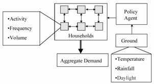
Figure 17. The structure of the water demand model
The neighbours in this model are those in the n spaces in the squares orthogonally adjacent to a household. The default value of this distance, n, was 4. The purpose of this neighbourhood shape was to produce a more complex set of neighbour relations than would be produced using a simple distance-related one as in the Schelling model (Figure 1), but still retain the importance of the influence of neighbours.
Figure 18. The neighbourhood pattern for the households
To give an idea of the social topology that results from this neighbourhood I have shown the “most similar” neighbour influence pattern at a point in a typical run of the model in Figure 19. Due to the fact that every neighbour has a unique most neighbour who is most influential to it, the topology of this social network consists of a few pairs of mutually most influential neighbours and a tree of influence spreading out from these. The extent of the influence that is transmitted over any particular path of this network will depend upon the extent each node in the path is biased towards being influenced by neighbours.
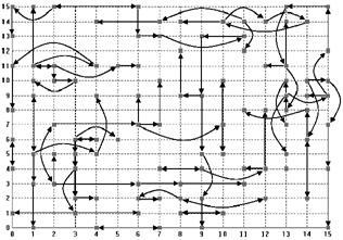
Figure 19. The most influential neighbour relation at a point in time during a typical run of the water demand model
Households are also (to a lesser extent) also influenced by all its neighbours in its neighbourhood (the one shown in Figure 18 above). Figure 20 illustrates all the effective neighbour relations between the households for the same instance. Note that the edges of this are not wrapped around into a torus in the examples described, so the households at the edges and corners have fewer neighbours that those in the middle. The reason for the chosen neighbourhood pattern is that the resulting patterns (as in Figure 19 above and Figure 1 above) seem to us a reasonable mix of locality and complexity. We have no good empirical basis for this, it just seems intuitively right to us and we could not find any evidence as to what the structure might be. I return to this issue in the discussion below.
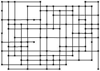
Figure 20. The totality of neighbour relations in the same case as Figure 19 (each node connects to those 4 up, down, left and right along the indicated lines)
In each run the households are distributed and initialised randomly, whilst the overall distribution of the ownership and usages of appliances by the households and the biases of the households is approximately the same. In each run the same weather data is used, so droughts will occur at the same time and hence the policy agent will issue the same advice. Also in each run the new innovations (e.g. power showers) are introduced at the same date. Figure 21 shows the aggregate water demand for 10 runs of the model with the same settings (normalised so that 1973 is scaled to 100 for ease of comparison).
To illustrate the difference when the social network is disrupted, I ran the simulation again with the same settings, social structures etc. except that whenever a household looks to other households, instead of perceiving that household’s (public) patterns of water use, the patterns of a randomly selected household is substituted. Thus the neighbour-to-neighbour influence is randomly re-routed in the second case. This is designed to be the minimal possible disruption of the social network, for it does not effect the number of neighbours of each household, their cognition, or the external factors – these all remain the same. Figure 22 shows 12 runs of this version of the model, this can be compared to Figure 21 where influence transmission is normal.
Figure 21. The aggregate water demand for 10 runs of the model (55% Neighbour biased, historical scenario, historical innovation dates, dashed lines indicate major droughts, solid lines indicate introduction of new kinds of appliances)
Figure 22. The aggregate water demand for 12 runs of the model where the neighbour relation is broken by randomisation
The qualitative difference between the two runs is reasonably clear. In the first set (Figure 21) there is an almost uniform reaction to droughts (i.e. the advice of the policy maker), with almost all runs showing a reduction in water demand during these periods, whilst in the second (Figure 22) the reaction to such periods is not a general reduction in demand but rather a period of increased volatility in demand. Secondly, the first set (Figure 21) shows a much greater stability than the second (Figure 22), which exhibits short term “oscillations” in demand.
What seems to be occurring is that in the first model small, denser neighbourhoods mutually influence each other to a certain pattern, damping down any avalanches of influence that may otherwise occur. In the disrupted case households “flip” between different patterns as the incoming perceived patterns vary, resulting in a lot of “noise” – this noise acts to drown out the relatively “faint” suggestions of the policy agent. I would guess that a “mean field” style social influence model, where each household perceives the average of its neighbour’s water use patterns would be even smoother and more consistent than the original model. Thus the social influence in the model can be seen as somewhere “between” that of the randomised and the “mean-field” abstract models, a situation which allows for localised, mutually reinforcing patterns of behaviour to compete with and influence other localised patterns of water use.
Elsewhere Barthelemy (2003) showed that the output of this model was qualitatively and significantly effected by different changes to the topology of the social network, including a change in the density of agent, whether the space has edges or not (i.e. whether the grid is toroidally wrapped around to iteself or not); and the size of the agent neighbourhoods.
In any case it is clear that the social network does have a significant effect upon the resulting behaviour of the simulation. In other work on this model it is clear that changing the distribution of biases on the household (so that more or less are biased towards being influenced by their neighbours or the policy agent) also changes the qualitative nature of the aggregate water demand patterns that result.
Discussion
One of the consequences of models such as those described above is that I have started to search for papers or researchers that may be able to give me some indication of how social and physical spaces are related in particular cases. Thus a natural question that arises in the model of social influence and domestic water use is what are the external influences upon households are – do they look to their immediate neighbours for cues to what is socially acceptable or does such influence spread mainly through local institutions such as the school, the pub or the place of work? However, as far as I can tell not much is known about this. This points to an obvious “gap” in the field research – social networks do look at the structure of who talks to who, but does not relate this (as far as I can tell) to physical location – geographers do look at where people are located in space but do not generally investigate any social structure that is not based upon physical locality. There are some simple studies which start to touch upon this relation, (e.g. Sudman 1988, Wellman 1996), but these only start to touch upon a single aspect of the relation of social and physical space corresponding to the local bias parameter in the modified Schelling Model above.
Social network theory is a long established field that studies the properties of social networks from both theoretical (e.g. Watts 1999) and empirical approaches. However it tends to focus overmuch on the network as its abstraction of choice, largely leaving out the cognition of the agent (Carley 2003). Thus social network theory complements that of cellular automata which is an abstraction of physical action (e.g. Pohill et al. 2001). Combining the two would lead to a richer and more complete model of many situations, however the interaction of physical and social space occurs primarily through the cognition of the agent. Thus to combine these two spaces one needs a modelling tools that also allows the representation of this cognition, i.e. an agent-based model.
Conclusion
If we are to take the physical and social embeddedness of actors seriously we need to model their interactions in both of these “dimensions” – assuming these away to very abstract models will lead to different, and possibly very misleading, results. Agent-based simulation seems to be the only tool presently available that can adequately model and explore the consequences of the interaction of social and physical space. It provides the “cognitive glue” inside the agents that connects physical and social spaces. Statistical and mathematical tools are not well suited to this task, but now we have the tool of agent-based simulation. Thus, perhaps for the first time, it is no longer necessary to “simplify away” all of the real contingencies of social interaction but start to capture these in descriptive social simulations. Such models will then allow a more informed determination of when and how abstraction can safely be done – until then, we may find all sorts of interesting properties of networks and structures, but we will have no evidence as to whether they are relevant other than their intuitive appeal.
Thus I am saying more than just that either: that there are aspects that are not covered in simpler models; or that an approach that starting with a model that is descriptively adequate to the available evidence is likely to be more productive than one that tries to start simply, i.e. a KIDS rather than a KISS approach as I advocate elsewhere (Edmonds 2004); but that models such as those above provide evidence that assuming-away the structure of the social network (that is separate from the physical topology) is dangerous. Thus the burdon of proof is upon those that make this kind of simplifying assumption to show that such assumptions are, in fact, justified. So far I have not seen any such evidence, and so one must conclude that any such work is likely to be inadequate to capture the essence of many occuring socially self-organised processes.
Acknowledgements
Thanks to the many people with whom I have discussed this subject, including: Scott Moss, David Hales, Tom Downing, Nick Gotts, and Olivier Barthelemy. Thanks also to Francesco Billari, Thomas Fent, Alexia Prskawetz, Jürgen Scheffran and Ani Gragossian, the organisers and secretary of the Topical Workshop on Agent-Based Computational Modelling, who invited me.
References
Carley, K. (2003) Dynamic Network Theory, In ….
Downing, T.E, Butterfield, R.E., Edmonds, B., Knox, J.W., Moss, S., Piper, B.S. and Weatherhead, E.K. (and the CCDeW project team) (2003). Climate Change and the Demand for Water, Research Report, Stockholm Environment Institute Oxford Office, Oxford. (http://www.sei.se/oxford/ccdew/)
Edmonds, B. (1999) Capturing Social Embeddedness: a Constructivist Approach. Adaptive Behaviour 7:323-348.
Edmonds, B. and Hales, D. (2003) Computational Simulation as Theoretical Experiment, CPM report 03-106, MMU, UK. (http://cfpm.org/cpmrep106.html)
KISS to KIDs
Edmonds, B. Barthelemy, O. and Moss, S. (2002) Domestic Water Demand and Social Influence – an agent-based modelling approach, CPM Report 02-103, MMU, 2002 (http://cfpm.org/cpmrep103.html).
Granovetter, M. (1985) Economic-Action and Social-Structure – The Problem of Embeddedness. American Journal Of Sociology 91:481-510.
Moss and Edmonds
Polhill, J.G. , Gotts, N.M. and Law, A.N.R. (2001) Imitative Versus Non-Imitative Strategies in a Land Use Simulation. Cybernetics and Systems 32:285-307.
Schelling, T. (1969) Models of Segregation. American Economic Review 59:488-493.
Sudman, S. (1988) Experiments in Measuring Neighbor and Relative Social Networks. Social Networks 10:93-108.
Watts, D. J. (1999) Small Worlds: The Dynamics of Networks between Order and Randomness. Princeton University Press.
Wellman, B. (1996) Are personal communities local? A Dumptarian reconsideration. Social Networks 18:347-354.