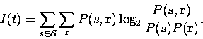
Abstract.Is the information transmitted by an ensemble of neurons determined solely by the number of spikes fired by each cell, or do correlations in the emission of action potentials also play a significant role? We derive a simple formula which enables this question to be answered rigorously for short timescales. The formula quantifies the corrections to the instantaneous information rate which result from correlations in spike emission between pairs of neurons. The mutual information that the ensemble of neurons conveys about external stimuli can thus be broken down into firing rate and correlation components. This analysis provides fundamental constraints upon the nature of information coding - showing that over short timescales, correlations cannot dominate information representation, that stimulus-independent correlations may lead to synergy (where the neurons together convey more information than they would considered independently), but that only certain combinations of the different sources of correlation result in significant synergy rather than in redundancy or in negligible effects. This analysis leads to a new quantification procedure which is directly applicable to simultaneous multiple neuron recordings.
Introduction
A controversy exists over the extent to which firing rates and correlations between the responses of different cells (such as synchronisation of action potentials) contribute to information representation and processing by neural ensembles. Encoding of information in the correlation between the firing of different neurons has been demonstrated in specialised sensory systems such as the salamander retina (Meister et al.; 1995) and the auditory localisation system of the barn owl (Carr and Konishi; 1990; Carr; 1993). For the mammalian cortex, the evidence is less clear. Several investigators (Singer et al.; 1997; Vaadia et al.; 1995; deCharms and Merzenich; 1996) have presented evidence of stimulus-related changes in the correlation of firing between small populations of cortical cells. This might imply that correlations among cortical neurons reveal a substantial capability of cortical neural ensembles to code information synergistically - that is, that the ensemble of neurons provides more information than the simple sum of the contributions of the individual cells. Another possibility is that correlations actually limit rather than improve the information capacity of the population (Gawne and Richmond; 1993; Shadlen and Newsome; 1998; Zohary et al.; 1994). A third possibility is that correlations have no major effect on the efficiency of neural codes (Amit; 1997; Golledge et al.; 1996; Rolls and Treves; 1998). What is clearly needed in order to reconcile these viewpoints is a rigorous quantitative methodology for addressing the roles of both correlations and rates in information encoding.Information theory (Cover and Thomas; 1991; Shannon; 1948), which has found much use in recent years in the analysis of recordings from single cells (Kitazawa et al.; 1998; Optican and Richmond; 1987; Rieke et al.; 1996; Rolls and Treves; 1998), provides the basis for such an approach. Ideally, it would be desirable to take any experiment in which population activity was recorded in response to a clearly identifiable stimulus which the cells participate in encoding, and determine how many bits of information were present in the firing rates, how many in coincident firing by pairs of neurons, etc. - to divide the information into components which are indicative of the information encoding mechanisms involved. By considering the limit of rapid information representation, in which the duration of the window of measurement is of the order of the mean inter-spike interval (ISI), it is possible to do just this. This short timescale limit is not only a convenient approach to a complex problem; it is likely to be of direct relevance to information processing by the brain, as there is substantial evidence that sensory information is transmitted by neuronal activity in very short periods of time. Single unit recording studies have demonstrated that the majority of information is often transmitted in windows as short as 20-50ms (Heller et al.; 1995; Macknik and Livingstone; 1998; Oram and Perrett; 1992; Rolls and Tovee; 1994; Tovée et al.; 1993; Werner and Mountcastle; 1965). Event related potential studies of the human visual system (Thorpe et al.; 1996) provide further evidence that the processing of information in a multiple stage neural system can be extremely rapid. Finally, if one wishes to assess the information content of correlational assemblies which may last for only a few tens of milliseconds (Singer et al.; 1997), then appropriately short measurement windows must be used.
The current work describes the use of information theory to quantify the relative contributions of both firing rates and correlations between cells to the total information conveyed.
We report an expansion of the expression for mutual information to second order in time, show that the second order terms break down into those dependent on rate and those dependent upon correlation, and demonstrate that this can form the basis of a procedure for quantifying the information conveyed by simultaneously recorded neuronal responses. We show that with pairs of cells the approach works well for time windows several hundred milliseconds long, the time range of validity decreasing approximately inversely with population size. The expansion for the information shows that in short but physiological timescales, firing rates dominate information encoding when cell assemblies of limited size are considered, since correlations begin to contribute only with subleading terms. We find that the redundancy of coding is dependent upon the specific combination of the correlation in the number of spikes fired in the time window, which in the limit of short time windows measures the probability of coincident firing and thus the extent of synchronisation, and the correlation among mean response profiles to different stimuli. Furthermore, we observe that even stimulus-independent correlations may in some circumstances lead to synergistic coding.
Methods
THE INFORMATION CARRIED BY NEURONAL RESPONSES AND ITS SHORT TIMESCALE EXPANSION.
Consider a period of time beginning at t0,
of (short) duration t, in which a stimulus s is present. Let the
neuronal population response during this time be described by the vector
![]() ,
the number of spikes fired by each cell. Typically each
component will have value 0 or 1, and only rarely higher. We may
alternately describe the response by the firing rate vector
,
the number of spikes fired by each cell. Typically each
component will have value 0 or 1, and only rarely higher. We may
alternately describe the response by the firing rate vector
![]() ;
this is purely for mathematical convenience and does not imply
that we assume a firing rate code. In a typical cortical neurophysiology
experiment we might hope to have tens of such trials with the same
stimulus identification s. The stimuli considered are purely abstract:
the procedures detailed in this paper are applicable to a wide variety of
experimental paradigms. However, it may help to conceptualise the stimulus
as for example which object, of some set, is being viewed by the
experimental subject; indeed, data from such an experiment is examined
later in this paper. Consider the stimuli to be taken from a discrete set
;
this is purely for mathematical convenience and does not imply
that we assume a firing rate code. In a typical cortical neurophysiology
experiment we might hope to have tens of such trials with the same
stimulus identification s. The stimuli considered are purely abstract:
the procedures detailed in this paper are applicable to a wide variety of
experimental paradigms. However, it may help to conceptualise the stimulus
as for example which object, of some set, is being viewed by the
experimental subject; indeed, data from such an experiment is examined
later in this paper. Consider the stimuli to be taken from a discrete set
![]() with S elements, each occurring with probability P(s). The
probability of events with response
with S elements, each occurring with probability P(s). The
probability of events with response ![]() is denoted as
is denoted as
![]() ,
and the joint probability distribution as
,
and the joint probability distribution as
![]() .
.
Following Shannon (1948), we can write down the mutual information provided by the responses about the whole set of stimuli as
This assumes that the true probabilities
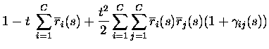
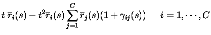
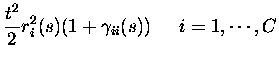
Now, the information can be approximated by a power series
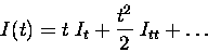
where It refers to the instantaneous information rate and Ittto the second time derivative of the information, the instantaneous information ``acceleration''. For short timescales, only the first order and second order terms survive - higher order terms in the series become negligible. The time derivatives of the information can be calculated by taking advantage of the short time limit, as we will explain.
DEFINITIONS AND MEASUREMENT OF CORRELATIONS FOR SHORT TIMESCALES.
There are two kinds of correlations that influence the information. These
have been previously termed ``signal'' and ``noise'' correlations
(Gawne and Richmond; 1993). They can be distinguished by separating the responses into
``signal'' (the average response to each stimulus) and ``noise'' (the
variability of responses from the average to each stimulus). The correlations in the
response variability represent the tendency of the cells to fire more (or
less) than average when a particular event (e.g. a spike from another
neuron) is observed in the same time window. For short time windows, this
of course measures the extent of synchronisation of the cells. One way to
introduce the parameters
![]() quantifying noise correlation in
the short time limit is in terms of the conditional firing probabilities:
quantifying noise correlation in
the short time limit is in terms of the conditional firing probabilities:
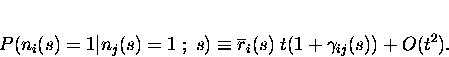
where
For ![]() ,
Eq. 3 gives us the probability
of coincident firing: cells i and j both fire spikes in the same time
period;
,
Eq. 3 gives us the probability
of coincident firing: cells i and j both fire spikes in the same time
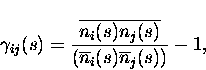
period;
![]() is the fraction of coincidences above (or below)
that expected from uncorrelated responses, normalised to the number of
coincidences in the uncorrelated case (which is
is the fraction of coincidences above (or below)
that expected from uncorrelated responses, normalised to the number of
coincidences in the uncorrelated case (which is
![]() ,
the bar denoting the average
across trials belonging to stimulus s).
,
the bar denoting the average
across trials belonging to stimulus s).
![]() is
thus given by the following expression:
is
thus given by the following expression:
 |
(4) |
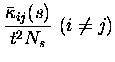
and is named the ``scaled cross correlation density'' (Aertsen et al.; 1989). It can vary from -1 to
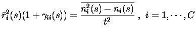
For i=j, Eq. (3) provides instead the probability of observing a spike emission by cell i given that we have observed a different spike from the same cell i during the same time window. The ``scaled autocorrelation coefficient'' must be measured as
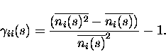 |
(5) |
Notice that in the numerator of the above equation the subtraction of
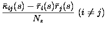
In order to maintain homogeneity with respect to the noise correlation
case, we choose to quantify the correlations in the signal, i.e. the
correlations ![]() in the mean responses of the neurons across the
set of stimuli, as a signal scaled crosscorrelation coefficient:
in the mean responses of the neurons across the
set of stimuli, as a signal scaled crosscorrelation coefficient:

The definition is similar to that of scaled noise correlation; the main difference is that now the average is across stimuli:
RESPONSE PROBABILITY QUANTIFICATION.
If the firing rates conditional upon the firing of other neurons are
non-divergent, as assumed in eq. (3), the texpansion of response probabilities becomes essentially an expansion in
the total number of spikes emitted by the population in response to a
stimulus. The only responses with non-zero probabilities up to order tkare the responses with up to k spikes from the population; the only
events with non-zero probability are therefore to second order in tthose with no more than two spikes emitted in total:
where
BIAS CALCULATION.
The information rate It and each of the three components of Ittare affected by a systematic error when calculated from limited data samples. This is a problem general to all nonlinear functions of probabilities, but has been noted to be of particular concern for Shannon information, from which It and Itt derive. Furthermore, the bias in the n-th derivative of the information has a 1/tn dependence, making treatment of the bias problem even more crucial. The problem can be largely avoided by estimating the bias by a standard error propagation procedure and subtracting it from the calculated quantity. The procedure is detailed in Appendix B.
INTEGRATE AND FIRE SIMULATION.
Correlated spike trains were simulated using a method similar to that used by Shadlen and Newsome (1998), to which we refer for a full discussion of the advantages and limitations of the model. In brief, each cell received 300 excitatory and 300 inhibitory inputs, each a Poisson process in itself, whose (possibly stimulus dependent) mean rate is constant across the set of inputs for any specific stimulus condition, and contributed a fixed quantity to the membrane potential, which decayed with a time constant of 20ms. When the membrane potential exceeded a threshold, it was reset to a baseline value. Crosscorrelation between cells was controlled through the proportion of inputs shared between cells (33% for Fig. 2b-c and 0%/90% for Fig. 2d-f). The spiking threshold was 14.5 times the magnitude of the quantal input above the baseline for the figures shown. The threshold and time constant parameters were chosen so as to guarantee the conservation of the response dynamic range, i.e. the neurons respond with approximately the same firing rate as their inputs over the range of cortical firing frequencies. Despite its simplicity, this ``Integrate and Fire'' model with balanced excitation and inhibition can account for several aspects of the firing statistics observed in responses of neurons across large regions of the cerebral cortex (Shadlen and Newsome; 1998).
By fixing the proportion of shared connections, but varying the mean firing rate according to which stimulus is present, rate coding in the presence of a fixed level of correlation can be examined. The mean firing rates chosen for each stimulus were extracted from data recorded from real inferior temporal cortical cells (see below). By holding the mean rate fixed (at the global mean corresponding to the previous case) but instead varying the proportion of shared connections according to the stimulus, one can examine a pure correlational code - thus allowing a clarification and test of the present information theoretic analysis.
Results
THE INFORMATION IN NEURONAL ENSEMBLE RESPONSES IN SHORT TIME PERIODS.
In sufficiently short time windows, at most two spikes are emitted
from the population. Taking advantage of this, the response
probabilities can be obtained explicitly in terms of pairwise
correlations - triplet and higher order interactions do not
contribute (see Methods). Here we report the result of the insertion
of the response probabilities obtained in this limit into the Shannon
information formula (1): exact expressions quantifying
the impact of pairwise correlations on the information transmitted by
groups of spiking neurons. The information depends upon both the noise
correlations ![]() and the signal correlations
and the signal correlations ![]() .
.
In the short timescale limit, the first (It) and second (Itt)
information derivatives suffice to fully describe the information
kinetics. The instantaneous information rate is

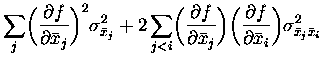
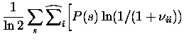
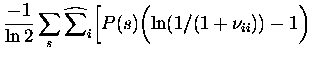
Note that the expression for It is just a generalisation to the population level (a simple sum) of the expression previously derived for single cells (Bialek et al.; 1991; Skaggs et al.; 1993). The expression for the instantaneous information acceleration breaks up into three terms
![$\displaystyle {1\over \ln 2} \sum_{i=1}^C \sum_{j=1}^C
\left<\overline {r}_{i}(...
...\right>_{s} \biggl[
\nu_{ij} + (1 + \nu_{ij})\ln ({1\over 1+\nu_{ij}} ) \biggr]$](img38.gif)
![$\displaystyle \sum_{i=1}^C \sum_{j=1}^C \biggl[ \left< \overline{r}_{i}(s)
\overline{r}_{j}(s)
\gamma_{ij}(s) \right>_s
\biggr] \log_2 ({1\over 1+\nu_{ij}})$](img39.gif)
![$\displaystyle \sum_{i=1}^C \sum_{j=1}^C \left< \overline{r}_{i}(s)
\overline{r}...
...(s')
\overline{r}_{j}(s')(1+ \gamma_{ij}(s'))\right>_{s'} } \biggr] \right>_s .$](img40.gif)
The first of these terms is all that survives if there is no noise correlation at all. Thus the rate component of the information is given by the sum of It (which is always greater than or equal to zero) and of the first term of Itt (which is instead always less than or equal to zero). The second term is non-zero if there is some correlation in the variance to a given stimulus, even if it is independent of which stimulus is present; this term thus represents the contribution of stimulus-independent noise correlation to the information. The third component of Itt represents the contribution of stimulus-modulated noise correlation, as it becomes non-zero only for stimulus-dependent correlations. We refer to these last two terms of Itt together as the correlational components of the information.
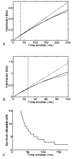
The result just described shows that the short timescale limit allows a rigorous quantification of the effect of correlations on the information conveyed by neuronal ensembles. The price to pay is the limited temporal range of applicability, as it formally requires that the mean number of spikes in the considered time window be small. What must now be addressed is the actual temporal range of applicability of the approach. The range of validity of the (order t2) approximation will depend on how well the information time dependence fits a quadratic approximation (e.g., for a quadratic function, the Taylor expansion to the second order would of course be exact for the entire t range). Since the assumption about the number of spikes will be broken first by the stimulus that gives the maximal response, a good scale for comparison with the range of validity is the minimum mean interspike interval to any stimulus. We studied the range of validity of the approximation, in the case of cells firing with Poisson statistics by direct calculation of the information; and in the more general case of up to four Integrate and Fire simulated neurons by a ``brute-force'' calculation, using many trials of simulated data. Fig. 1a shows the accuracy of the approximation for a pair of Poisson-simulated cells with mean-rate characteristics of real inferior temporal (IT) cells (Booth and Rolls; 1998); the range of validity in this case would appear to be, being conservative, about 6-8 times the minimum mean interspike interval. The approximation is better for smaller samples of cells. Scaling considerations suggest that the range of applicability should shrink as the inverse of the number of cells for larger populations. This expectation is roughly confirmed by the results in Fig. 1b, where five Poisson cells (again with typical cortical firing rates) are analysed. Integrate and Fire simulations confirm that this estimate of the range of validity is relatively robust to neuronal statistics and conserved across a wide range of response correlation values. Fig. 1c shows an estimate of the allowed ensemble size versus the time window for cells with mean rates to stimuli extracted from the cortical data of (Booth and Rolls; 1998). We conclude that the analysis is pertinent for timescales relevant to neuronal coding for ensembles of up to around 10-15 cells with firing rates similar to those in inferior temporal cortex, and for even larger ensembles of cells with lower firing rates, such as medial temporal lobe cells.
|
RATE AND CORRELATION COMPONENTS OF THE INFORMATION.
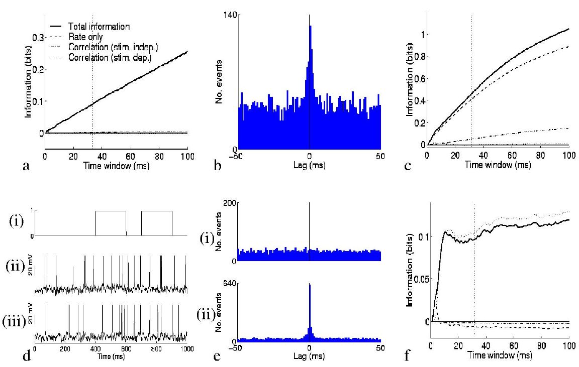
So what is the impact of the second order terms on the information conveyed by the ensemble of neurons? Fig. 2 provides an illustration of their effect. In the case of non-interacting cells with zero autocorrelation, the information is carried entirely in the rate component of the information. This was exemplified by simulating a quintuplet of cells, each of which fired spikes according to a Poisson process (at any instant in time there is a given probability of firing which is constant in time throughout the experimental trial), independently of other cells, with a mean rate which was different for each of ten stimuli. The mean rate profiles of each of the five cells were taken from real cells described in (Booth and Rolls; 1998); these real cells were the ones analysed as simultaneously recorded pairs later in the paper, facilitating comparison with the real data examined. The result is shown in Fig. 2a, which, like the other graphs, shows separately the contributions of the three terms to the total information. The last two of these (the contributions of correlations) are negligible in the example of Fig. 2a, since the spike trains were by design uncorrelated.
By simulating spike trains with the Integrate and Fire model,
we were able to examine situations in which
the correlational components of the information were not negligible. The
first such case considered was that of a quintuplet of neurons which had a
large amount of common input (one third of their connections were
shared). These neurons fired spikes in response to a balance of excitatory
and inhibitory input (see Methods), with a membrane decay time of 20
milliseconds leading to a small amount of correlated firing, as shown by
the crosscorrelogram in Fig. 2b. Ten stimuli again induced different mean
firing rate responses from the cells. The correlation is not
stimulus-dependent, and therefore the third component of Itt is still
zero in this case. The second component of Itt, representing the
effect of stimulus-independent correlation, can if required be again
broken up into auto- (i=j) and cross-correlation (![]() )
parts. The
elements corresponding to autocorrelation are always positive for
autocorrelations
)
parts. The
elements corresponding to autocorrelation are always positive for
autocorrelations
![]() between -1 and 0 (as observed for the IT
cells), whereas the crosscorrelation component is positive when, for
positive noise correlation, the signal correlation is negative, i.e. when
the cells anti-covary in their stimulus response profiles. In the case
shown in Fig. 2c, this term is positive, and leads to a modest increase in
the total information that can be transmitted.
between -1 and 0 (as observed for the IT
cells), whereas the crosscorrelation component is positive when, for
positive noise correlation, the signal correlation is negative, i.e. when
the cells anti-covary in their stimulus response profiles. In the case
shown in Fig. 2c, this term is positive, and leads to a modest increase in
the total information that can be transmitted.
To model a situation where stimulus-dependent correlations conveyed information, we generated simulated data using the Integrate and Fire model for another quintuplet of cells which had a stimulus-dependent fraction of common input. This might correspond to a situation where cells transiently participate in different neuronal assemblies depending on stimulus conditions. There were again ten stimuli, but this time the mean spike emission rate to each stimulus was constant, at approximately 20 Hz, the global mean firing rate for the previous case. One of these stimuli simply resulted in independent input to each of the model cells, whereas each of the other nine stimuli resulted in an increase (to 90%) in the amount of shared input between one pair of cells (chosen at random from the ensemble such that each stimulus resulted in a different pair being correlated). The response of one such pair to changes in the amount of common input is shown in Fig. 2d. Panel (i) shows the fraction of shared connections as a function of time; panels (ii) and (iii) show the resulting membrane potentials and spike trains from the pair of neurons. During the high correlation state, there was on average 7 times higher probability of a coincidence in any 10ms period than chance. This crosscorrelation is also evident in the crosscorrelograms shown in Fig. 2e. The results are given in Fig. 2,,,f: all terms but the third of Itt are essentially zero, and information transmission is in this case almost entirely due to stimulus-dependent correlations. The total amount of information that could be conveyed, even with this much shared input, was modest in comparison to that conveyed by rates dependent on the stimuli, at the same mean firing rate. The total information increased slightly if for the ``high correlation'' state the spike trains were nearly perfectly correlated; if the ``low correlation'' state corresponded not to chance, but to actual anticorrelation, then it is possible that even more information could be conveyed.
|
|
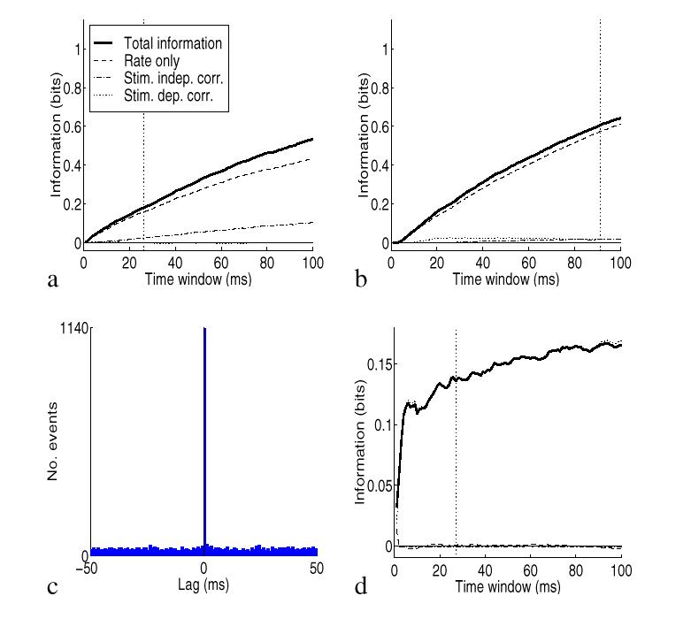
To illustrate the impact of the population size and of the overall average firing rate, we performed more simulations using again the spike trains with the Integrate and Fire model with a time constant of 20 ms and 30% shared connections, as in Fig. 2b,c. In Fig. 3a we tested the effects of population size by computing the information from pairs of cells instead of from five cells, by extracting pairs from the set of five cells and then averaging across pairs. The effect of reducing the size of the population from five to two cells was to reduce the total information by a factor of about 2. It is of course expected that the amount of information depends on the number of cells in the population. It is also shown with this particular set of generated spikes that the relative amount of information in the different components is approximately similar. In Fig. 3b we show the effects of applying the methods to cells with lower firing rates. The lower firing rates were produced simply by dividing the rates by three relative to those used in Fig. 2c. (This places the firing rates of the cells in the same regime as that of primate hippocampal pyramidal neurons in vivo, which fire at lower rates than cortical visual cells (Rolls, Robertson and Georges-François; 1997).) The information was computed from the responses of the population of five simulated cells. The effect of dividing the overall firing rate by three was to reduce the information by approximately two. If only the first derivative was important, we would expect the total information to decrease linearly when decreasing the rate. The sublinear decrease is mostly due to the rate component of the second derivative, which is a negative contribution, larger for higher rates and much smaller for lower rates. Similarly, the correlational component of the information is also much less important for lower rates, as evident from our analysis.
To illustrate the effects of precision of synchrony, we produced spike trains by simulating a correlational assembly with a constant firing rate of 20 Hz to all stimuli, and a percentage of shared connections of either 0% or 90% to different stimuli. In order to increase the precision of the synchrony with respect to Fig. 2d-f, we decreased the membrane time constant to the value of 1 ms. This gives, in the high correlation state, a very precise 1 ms synchrony between the spike trains, as shown by the crosscorrelogram in Fig. 3c. The information, shown in Fig. 3d, is fully conveyed by the correlational component with no information in the firing rates, correctly reflecting the way in which the spikes were generated. The actual information with the 1 ms precision is higher by a factor of 1.5 with respect with the 20 ms membrane time constant (Fig. 2f). Thus the precision of spike synchrony has an impact on the correlational part of the information, as predicted by our analysis.
|
|
APPLICATION OF THE METHOD TO REAL NEURONAL DATA
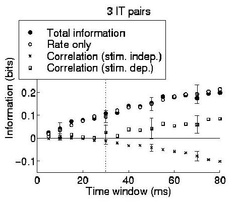
To demonstrate that the technique is applicable to real data, we applied the information component analysis to three pairs of cortical cells recorded simultaneously from the same electrode from the dataset of (Booth and Rolls; 1998). This data came from an experiment in which the responses of neurons in the inferior temporal cortex of the macaque monkey were recorded while one of ten different objects was being viewed. The firing rates of these neurons were found by Booth and Rolls (1998) to convey information about which object was present, regardless of viewing angle. Four different views of each object were each presented five times, resulting in a total of twenty trials for each object. The median firing rate to the best stimulus of the cells used in our analysis was 44 Hz. The same data was used to estimate realistic firing rates for all the simulations described in this paper.
Each component of the information for the cells in this dataset were calculated for each pair of cells, and the standard error in the calculation of each information component was obtained by error propagation from the variances in the measurements of spike counts and coincidences over the trials. The average information encoding characteristics of the three pairs (which were qualitatively similar to each other) is shown in Fig. 3. In this example it is clear that the rate component is prominent in the information representation; however, the important point to gain from this result is that the information expansion provides a demonstrably practical method for analysing simultaneously recorded data with only a small number of experimental trials. The values of each component and an estimate of its error are available both for single small ensembles, and for the ``average picture'' obtained by recording large numbers of such small neuronal ensembles. This encourages us to think that it will be possible to analyse simultaneously recorded data in a systematic and rigorous quantitative manner. Of course, the populations of neurons that actually act effectively together are larger than can be studied using this, or any other presently known procedure. However, it is reasonable to assume that effects present in such large ensembles will be to some extent observable in the smaller ensembles that we can in practice record from and analyse.
|
Discussion
REDUNDANCY VERSUS SYNERGY.
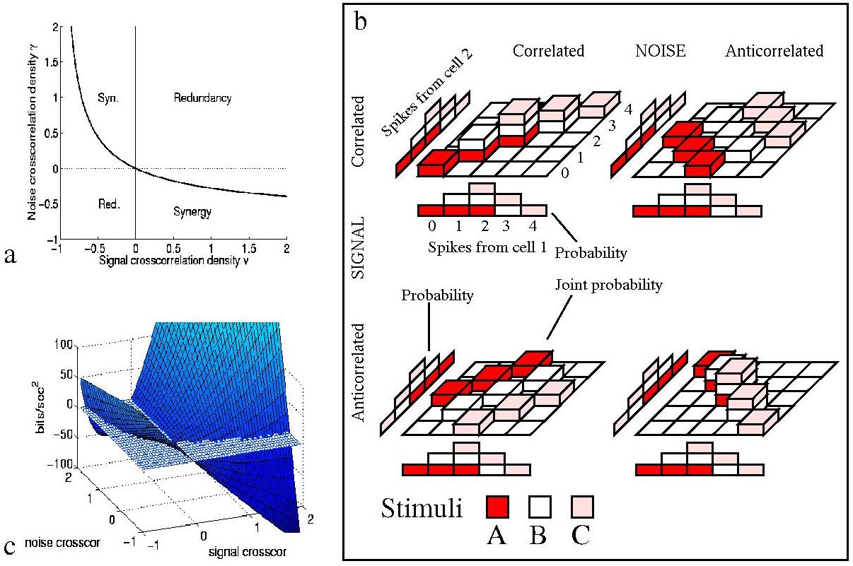
The redundancy of a code can be defined (and measured in bits) as the amount of information that would be obtained by adding the information obtained from each cell as if they were independent minus that obtained by considering the whole neuronal ensemble (Rieke et al.; 1996). (If part of what two neurons are saying is the same, it does not help to say it twice.) For synergistic coding (in which knowledge of the states of a pair of neurons at the same time provides more information than one would obtain by considering each neuron alone), the value of this Shannon redundancy is of course negative.
Eq. 9 shows that overall correlations in the distribution
of mean responses alone can only lead to redundancy - since all (i,j)contributions to the first term of Itt are negative, except that they
are zero when there is no overall ``signal'' correlation in the mean
response profiles (i.e.
![]() ). To have synergistic coding of
information one needs correlations in the variability of the responses (to
a given stimulus), i.e. non-zero
). To have synergistic coding of
information one needs correlations in the variability of the responses (to
a given stimulus), i.e. non-zero ![]() parameters. Even when such
``noise'' correlations are independent of the stimuli, however, it is
possible to have synergy. This can be demonstrated by considering the sign
of the Shannon redundancy, obtained from Eq. 1 by
subtracting the information conveyed by the population from the sum of
that carried by each single cell. This shows four basic régimes of
operation, illustrated in the two-cell example of Fig. 5. If the cells
anti-covary in their response profiles to stimuli, the cell must have a
positive noise correlation, above the boundary value depicted in
Fig. 5(a), to obtain synergy; or if the cells do have positive signal
correlation, then coincidences must be actively suppressed by a negative
noise correlation stronger than the corresponding boundary value. When the
signal and noise correlations have the same sign, one always obtains
redundancy in the short timescale limit. Clearly, already with pairs of
cell, the interplay between correlation in the noise and correlation in
the signal introduces a potential for both redundancy and synergy.
parameters. Even when such
``noise'' correlations are independent of the stimuli, however, it is
possible to have synergy. This can be demonstrated by considering the sign
of the Shannon redundancy, obtained from Eq. 1 by
subtracting the information conveyed by the population from the sum of
that carried by each single cell. This shows four basic régimes of
operation, illustrated in the two-cell example of Fig. 5. If the cells
anti-covary in their response profiles to stimuli, the cell must have a
positive noise correlation, above the boundary value depicted in
Fig. 5(a), to obtain synergy; or if the cells do have positive signal
correlation, then coincidences must be actively suppressed by a negative
noise correlation stronger than the corresponding boundary value. When the
signal and noise correlations have the same sign, one always obtains
redundancy in the short timescale limit. Clearly, already with pairs of
cell, the interplay between correlation in the noise and correlation in
the signal introduces a potential for both redundancy and synergy.
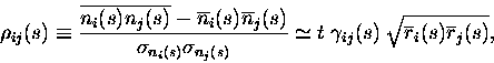
A simple example of the interplay between signal and noise correlation in
a pair of cells is graphically depicted in Fig. 5(b). In this example
there are three stimuli, A, B and C, which occur with equal
probability. The first cell emits a different mean number of spikes to
each stimulus: 1 to A, 2 to B, and 3 to C. Let us consider cases where the
second cell either fires the same mean number of spikes to each stimulus
(full correlation), or alternatively has the mean responses to A and C
exchanged (anti-correlation with
![]() ). On any given occasion,
noise adds 0 or
). On any given occasion,
noise adds 0 or ![]() spikes, with equal (1/3) probability, to the
output of the cell. It is easy to check that the information carried by
each cell alone is
spikes, with equal (1/3) probability, to the
output of the cell. It is easy to check that the information carried by
each cell alone is
![]() bits, which is less than half
the
bits, which is less than half
the
![]() maximum information (entropy) available in the stimulus
set.
maximum information (entropy) available in the stimulus
set.
Fig. 5(b) illustrates the four different situations for the second cell,
depending on the way in which the mean (signal) and variance (noise) of
the number of spikes fired by it are related to those of the first
cell. When the signal and noise are both correlated (or both
anti-correlated), the joint probabilities of the numbers of spikes fired
by each cell tend to bunch up along the diagonal, so that the total
information from both cells is less than the sum of that obtained from
each cell on its own. If however with correlated signal the noise is
anti-correlated or if with correlated noise, the signal is
anti-correlated, then the joint probabilities are more spread out. This
means that the presented stimulus can be clearly identified on the basis
of the joint response observed. If this spread is sufficient, it is
possible to obtain synergy: the information calculated from the joint
probability matrix exceeds the sum of that obtained for each cell
individually. In this example, with the signal having
![]() (anti-correlation), if the noise was uncorrelated between the cells, then
the redundancy can be easily seen to be 0.04 bits; it is only when the
noise correlation is increased above
(anti-correlation), if the noise was uncorrelated between the cells, then
the redundancy can be easily seen to be 0.04 bits; it is only when the
noise correlation is increased above
![]() that the coding is
synergistic.
that the coding is
synergistic.
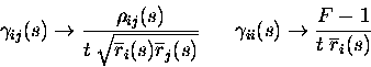
Examination of Eq.(9) and Fig. 5(c) reveals the total amount of redundancy (or synergy) to be much more sensitive to noise correlation when the signal correlation is high - e.g. the noise correlation leads to large redundancy if the cells are tuned to the same stimulus. If the signal correlation is small, the redundancy is close to zero, no matter how correlated the noise is. This explains why the impact of noise correlation on the performance of pools of neurons has been emphasised in experiments utilising simple one-dimensional discrimination tasks (in which neurons from a local pool have been found to be tuned to the same stimulus (Parker and Newsome; 1998; Zohary et al.; 1994)), while noise correlation has been described as less important for groups of neurons coding for complex stimuli (Gawne and Richmond; 1993; Gawne et al.; 1996), which tend to use a more distributed encoding. This study therefore shows rigorously that correlations do not necessarily invoke redundancy, and that it is not possible in general to estimate the `effective' number of neurons participating in encoding by simply measuring the noise correlation, as done by Zohary et al. (1994). Further, it predicts, since the signal correlation was reported to decrease towards zero when increasing the complexity of the stimulus set used to test the neurons (Gawne et al.; 1996; Rolls et al.; 1997), that noise correlation might have only a small impact in the encoding of large sets of natural stimuli - at least as far as stimulus-independent noise correlation is concerned. The effect of small stimulus-dependent correlations in the noise is considered below, and it should not be neglected.
The possibility of synergy with constant correlations has been raised previously (Oram et al.; 1998) as a phenomenological observation; the information expansion we have introduced places this phenomenon on a solid mathematical footing, and delineates, for short time windows, the exact boundaries of the regions of synergy and redundancy. The discussion by Oram et al. (1998) points out that correlations might lead to synergy when neurons are tuned to different stimuli, but it is not able to bridge between different encoding situations and predict the exact amounts of redundancy or synergy that occur, as our analysis does. The analysis of synergy presented here, unlike that of (Oram et al.; 1998), generalises to the case of stimulus-modulated correlations - it is enough to specify the stimulus dependence of correlations and take into account also the third term of Itt.
|
|
A NULL HYPOTHESIS FOR THE ROLE OF CORRELATIONS IN THE CEREBRAL CORTEX
How might typical correlations among cells in a population scale up with
the size of the population? Clearly, this is a question for experiments to
address, in fact a most crucial question for those investigating
correlations in neural activity.
Such experiments need to be well designed, accurate and systematic. It is
easy to see, from the analysis above, that with large populations even small
correlations could produce extreme effects, resulting in either large
redundancy or (perhaps less often) very substantial synergy. This is
because, while with C cells there are C first order terms in the
information, there are obviously C2 second order terms, C3 third order
ones (which depend also on three-way correlations) and so on. Depending
on tiny details of the correlational structure, successive terms can affect
transmitted information in both directions. Within such broad a realm
of possibilities, it is then of interest to try to formulate a sort of null
hypothesis, that might provide at least a reference point against which to
contrast any more structured candidate theory.
One example is the scaling behaviour we might expect if the
correlations were not playing any special role at all in the
system or area being analysed. In this ``null'' hypothesis, the parameters
![]() would be expected to be small, that is to deviate from 0 (no
correlations) only in so far as the set of stimuli used is limited
(Gawne and Richmond; 1993; Rolls, Treves and Tovée; 1997); similarly the stimulus-dependent noise
correlation
would be expected to be small, that is to deviate from 0 (no
correlations) only in so far as the set of stimuli used is limited
(Gawne and Richmond; 1993; Rolls, Treves and Tovée; 1997); similarly the stimulus-dependent noise
correlation
![]() would be small. The scaling behaviour
corresponding to this null hypothesis can be examined by further expanding
Itt as a series in these new small parameters: at times of the order
of the inter-spike interval, second order terms of order
would be small. The scaling behaviour
corresponding to this null hypothesis can be examined by further expanding
Itt as a series in these new small parameters: at times of the order
of the inter-spike interval, second order terms of order
![]() (redundant) and
(redundant) and
![]() (synergistic) are introduced (the angular brackets
indicating the average value). If we have a large enough population of
cells, and
(synergistic) are introduced (the angular brackets
indicating the average value). If we have a large enough population of
cells, and
![]() and
and
![]() are
not sufficiently small to counteract the additional C factor, these
``random'' redundancy and synergy contributions will be substantial.
Obviously, in this situation our expansion would start to progressively
fail in quantifying the information, as higher order terms in the texpansion become more and more important in this case. But this clearly
shows that a sufficiently large population of cells, which has not been
designed to code stimuli in any particular cooperative manner, has the
potential to provide large effects of redundancy or synergy, arising
simply from random correlations among the firing of the different
cells. This reinforces the need for systematic study of the magnitude and
scaling of correlations in the cerebral cortex.
are
not sufficiently small to counteract the additional C factor, these
``random'' redundancy and synergy contributions will be substantial.
Obviously, in this situation our expansion would start to progressively
fail in quantifying the information, as higher order terms in the texpansion become more and more important in this case. But this clearly
shows that a sufficiently large population of cells, which has not been
designed to code stimuli in any particular cooperative manner, has the
potential to provide large effects of redundancy or synergy, arising
simply from random correlations among the firing of the different
cells. This reinforces the need for systematic study of the magnitude and
scaling of correlations in the cerebral cortex.
CORRELATIONAL ASSEMBLIES AND MUTUAL INFORMATION
If cells participate in context-dependent correlational assemblies (Singer et al.; 1997), then a significant amount of information should be found in the third component of Itt, relative to the total information, when analysing data obtained from the appropriate experiments. The challenge for the establishment of correlational theories of neural coding has thus been laid down: to demonstrate quantitatively how substantial a proportion of the information about external correlates is provided by correlations between cells, given the large amount of information that has been shown in some neural systems to be coded by rate (Rolls and Treves; 1998). The second order series expansion we have described allows precisely this to be achieved for small ensembles of cells - for a time window of 20ms, an ensemble of about 10-15 cells which fired at a peak mean rate to a stimulus of around 50Hz (e.g. IT cells) could be analysed; with the same time window, 25-30 cells firing at a lower peak mean rate of around 20 Hz, (such as neurons from the medial temporal lobe) could be studied. Beyond this population size the information expansion can still be of use in picking up the correlational variables conveying most of the information in small subpopulations, and eliminating the irrelevant variables. Reduction of the response space of a large population of cells to a treatable size thus may be possible without loosing salient features.
In order to test hypotheses about the role of correlations in solving the binding problem (Gray et al.; 1992; Singer et al.; 1997; von der Malsburg; 1995), as opposed to other solutions (Treisman and Gelade; 1980; Treisman; 1996), and about information coding in general (Vaadia et al.; 1995; deCharms and Merzenich; 1996), careful quantitative experimental studies of the correlations prevailing in the neural activity of different parts of the brain are needed. Data analyses based on the time-expansion approach then have the potential to elucidate the role of correlations in the encoding of information by cortical neurons.
Acknowledgements
We thank R. Baddeley, A. Renart and D. Smyth for useful discussions. We thank M. Booth for kindly providing neurophysiological data. This research was supported by an E.C. Marie Curie Research Training Grant ERBFMBICT972749 (SP), a studentship from the Oxford McDonnell-Pew Centre for Cognitive Neuroscience (SRS), and by MRC Programme Grant PG8513790.
Appendix A. Correlation measures.
The numerical value of the information calculated is independent of the correlation measure used, and we show here how to express the results using the Pearson correlation coefficients and Fano factors instead of scaled cross correlation coefficients. In the text, we chose to use the scaled cross-correlation measure of Eq. 3 because it produces a more compact mathematical formulation of what is addressed in this paper, and has useful scaling properties as the time window becomes small.
A widespread measure for crosscorrelation is the Pearson correlation
coefficient
![]() ,
which normalises the number of coincidences
above independence to the standard deviation of the number of
coincidences expected if the cells were independent. The normalization
used by the Pearson correlation coefficient quantifies the strength of
correlations between neurons in a rate-independent way. However, it
should be noted that the Pearson noise-correlation measure approaches
zero at short time windows:
,
which normalises the number of coincidences
above independence to the standard deviation of the number of
coincidences expected if the cells were independent. The normalization
used by the Pearson correlation coefficient quantifies the strength of
correlations between neurons in a rate-independent way. However, it
should be noted that the Pearson noise-correlation measure approaches
zero at short time windows:
 |
(10) |
where
Under assumption 3,
![]() remains finite as
remains finite as ![]() ,
thus by using this measure we can keep
the t expansion of the information explicit. This greatly increases
the amount of insight obtained from the series expansion.
,
thus by using this measure we can keep
the t expansion of the information explicit. This greatly increases
the amount of insight obtained from the series expansion.
Similarly, an alternative to scaled autocorrelation density
![]() for the measure of autocorrelations is the so called
``Fano'' factor F, that is the variance
of the spike count divided by its mean (Rieke et al.; 1996).
This measure is used in
neurophysiology because for the renewal process, often used as a
stochastic
model of neuronal firing, the variance is proportional to the mean.
(Fano factors lower than 1 indicate that the process is more regular
than a
Poisson process). F grows linearly with t for short
times:
for the measure of autocorrelations is the so called
``Fano'' factor F, that is the variance
of the spike count divided by its mean (Rieke et al.; 1996).
This measure is used in
neurophysiology because for the renewal process, often used as a
stochastic
model of neuronal firing, the variance is proportional to the mean.
(Fano factors lower than 1 indicate that the process is more regular
than a
Poisson process). F grows linearly with t for short
times:
![]() .
Again, we prefer
.
Again, we prefer
![]() to the Fano factor in the information expansion because F-1 approaches
zero for short times.
to the Fano factor in the information expansion because F-1 approaches
zero for short times.
To express the information derivatives in terms of Pearson correlation coefficients and Fano factor, is is enough to make the following simple substitutions in eq. (9):
 |
(11) |
We note that the ``scaled cross-correlation measure''
![]() is
sensitive to the mean firing rate, as the strength of neuronal
interactions might be
overemphasized at low rate (Aertsen et al.; 1989): it cannot be taken to be a
linear measure of interaction strength.
However, the value of the information transmitted by the the number of spikes
simultaneously fired by each cell, and of each particular components,
depends on the response probabilities, and not on the particular way chosen
to quantify the correlations. Therefore the particular measure used for
correlations is for this application ultimately a matter of mere notation.
is
sensitive to the mean firing rate, as the strength of neuronal
interactions might be
overemphasized at low rate (Aertsen et al.; 1989): it cannot be taken to be a
linear measure of interaction strength.
However, the value of the information transmitted by the the number of spikes
simultaneously fired by each cell, and of each particular components,
depends on the response probabilities, and not on the particular way chosen
to quantify the correlations. Therefore the particular measure used for
correlations is for this application ultimately a matter of mere notation.
Appendix B: Evaluation of the bias and of the variance of information derivatives
It is possible to analytically derive an estimate of the amount of the bias, which can then be subtracted to provide an unbiased estimate. This is done using the standard error propagation procedure (see e.g. Bevington and Robinson; 1992).
A function of the firing rates can be expanded about the mean rate as
 |
(1) |
where
| (2) |
Applying this to Eq. 8, we obtain
 |
(3) |
where the `hat' over the i summation indicates that it is only over the `relevant' s,i pairs, i.e. those with non-zero underlying probability of spike emission. If the underlying probability is zero, then no finite sampling fluctuations are possible and that s,i does not contribute to the bias.
Obviously this correction as it stands cannot be applied to the components
of Itt. A similar correction can be derived by the same method. This
calculation as we shall see is slightly more involved.
We will have to calculate the bias for each component of Ittseparately, so we will consider a generic function
![]() of a
set
of a
set
![]() of (possibly correlated) random variables. Each random
variable
of (possibly correlated) random variables. Each random
variable ![]() is the average (obtained on the basis of a limited
number of trials N) of a random variable xj. We assume for the
purposes of our analytical estimate that the number of trials N is large
but finite. In this case the independent variables
is the average (obtained on the basis of a limited
number of trials N) of a random variable xj. We assume for the
purposes of our analytical estimate that the number of trials N is large
but finite. In this case the independent variables
![]() fluctuate around their true value
fluctuate around their true value
![]() ,
and the fluctuations scale as 1/N.
Therefore this derivation of the bias of each information component
using error propagation is equivalent to the 1/N expansion of the bias
of the full information derived e.g. in (Panzeri and Treves; 1996).
,
and the fluctuations scale as 1/N.
Therefore this derivation of the bias of each information component
using error propagation is equivalent to the 1/N expansion of the bias
of the full information derived e.g. in (Panzeri and Treves; 1996).
Under these assumptions, the sampling
bias in
![]() is:
is:

where the (co)variances of the means of the random variables


The expression for the variance of
To apply the above formalism to our cases of the information derivative
components Itt1 - Itt3, the random variables used are the
![]() mean rates of the cells to each stimulus
mean rates of the cells to each stimulus
![]() ,
and the
,
and the
![]() variables
variables
![]() ,
which are defined as
,
which are defined as
| = |  |
(8) | |
| = |  |
(9) |
The leading contributions of these (co)variances can be calculated
analytically in the short time window limit.
They are:


Note that the leading order fluctuations are those in the number of coincidences (i.e.
Carrying out the differentiation, we obtain for the bias of the three
separate components of Itt (denoted by
Itt1(bias),Itt2(bias), Itt3(bias)):

![$\displaystyle \widehat{\sum}_j {\bar{r}^2_j(s) \over < \bar{r}_i(s')\bar{r}_j(s...
...\bar{r}_j(s') >_{s'} \over \bar{r}^2_i}
\biggr) \biggr] \sigma^2_{\bar{r}_i(s)}$](img105.gif)


![$\displaystyle P(s)\widehat{\sum}_j {<\bar{\kappa}_{ij}(s')>_{s'} \bar{r}_j^2(s)...
...\bar{r}_i^2(s) \over
<\bar{r}^2_i(s') >_{s'}^2}
\biggr] \sigma^2_{\bar{r}_i(s)}$](img109.gif)


The `hats' in the summations of terms proportional to
Note that the leading contribution to the Itt bias is from Itt3, which is proportional to 1/t2, whereas the biases in Itt1 and Itt2 are only proportional to 1/t.
We now have analytical expressions for the bias due to finite sampling in each of the components of Itt, as well as It. The bias estimate obtained from each of these is subtracted from the `raw' quantity. A more detailed study of the range of validity of the bias removal using simulated data can be found in (Schultz; 1998).
We conclude by noting that the procedure used to count `bins' for the summation over `relevant bins' in the above equations was a `naive' counting procedure, in which we only add terms in which there is at least one spike (or coincidence if it is a sum over i and j) in any of the trials. For sufficiently short time windows, and a small number of trials per stimulus, the bias correction fails. This occurs more evidently in Itt3 because of the 1/t2 dependence. Other non-naive counting procedures can be used to obtain more accurate estimates of the bias. By using a Bayesian counting procedure (exactly the same one described in (Panzeri and Treves; 1996)), it was possible to reduce somewhat the time at which the bias correction broke down, and obtain a more accurate bias estimation at very short times, at the expense of losing the property that the resulting information estimate is an upper bound on the information. In this procedure, the problem of the summations reduces to estimating the number of relevant bins. This is done by choosing a ``guess'' value for the number of relevant bins, and a prior probability function which has one (constant) value for each of the occupied bins and another (constant) value for each of the empty bins. The posterior probability distribution is then calculated and the posterior estimate of the number of relevant bins obtained. This procedure applies just as well to Itt3 as it did to the full information in the case described by Panzeri and Treves (1996). We do not describe this Bayesian counting procedure here, because it is exactly the one reported in Panzeri and Treves (1996); however, for values of firing rates in the range relevant for visual cortical cells, the use of a Bayesian counting procedure makes a difference only for time windows as short as 2-3 ms.
References
- Aertsen, A. M. H. J., Gerstein, G. L., Habib, M. K. and Palm, G. (1989).
-
Dynamics of neuronal firing correlation: modulation of ``effective
connectivity'', J. Neurophysiol. 61: 900-917.
- Amit, D. J. (1997).
-
Is synchronization necessary and is it sufficient?, Behavioural
and brain sciences 20: 683.
- Bevington, P. R. and Robinson, D. K. (1992).
-
Data Reduction and error analysis for the physical sciences, McGraw-Hill, New York.
- Bialek, W., Rieke, F., de Ruyter van Steveninck, R. R. and Warland, D. (1991).
-
Reading a neural code, Science 252: 1854-1857.
- Booth, M. C. A. and Rolls, E. T. ( 1998).
-
View-invariant representations of familiar objects by neurons in the
inferior temporal visual cortex, Cerebral Cortex 8: 1047-3211.
- Carr, C. E. (1993).
-
Processing of temporal information in the brain, Ann. Rev.
Neurosci. 16: 223-243.
- Carr, C. E. and Konishi, M. (1990).
-
A circuit for detection of interaural time differences in the
brainstem of the barn owl, J. Neurosci. 10: 3227-3246.
- Cover, T. M. and Thomas, J. A. (1991)
- .
Elements of information theory, John Wiley, New York.
- deCharms, R. C. and Merzenich, M. M. ( 1996).
-
Primary cortical representation of sounds by the coordination of
action potentials, Nature 381: 610-613.
- Gawne, T. J., Kjaer, T. W., Hertz, J. A. and Richmond, B. J. (1996).
-
Adjacent visual cortical complex cells share about 20% of their
stimulus-related information, Cerebral Cortex 6: 482-489.
- Gawne, T. J. and Richmond, B. J. ( 1993).
-
How independent are the messages carried by adjacent inferior
temporal cortical neurons?, J. Neurosci. 13: 2758-2771.
- Golledge, D. R., Hildetag, C. C. and Tovée, M. J. (1996).
-
A solution to the binding problem?, Current Biology 6(9): 1092-1095.
- Gray, C. M., Engel, A. K., König, P. and Singer, W. (1992).
-
Synchronization of oscillatory neuronal responses in cat striate
cortex: Temporal properties, Visual Neuroscience 8: 337-347.
- Heller, J., Hertz, J. A., Kjaer, T. W. and Richmond, B. J. (1995).
-
Information flow and temporal coding in primate pattern vision, J. Comp. Neurosci. 2: 175-193.
- Kitazawa, S., Kimura, T. and Yin, P.-B. ( 1998).
-
Cerebellar complex spikes encode both destinations and errors in arm
movements, Nature 392: 494-497.
- Macknik, S. L. and Livingstone, M. S. ( 1998).
-
Neuronal correlates of visibility and invisibility in the primate
visual system, Nature Neuroscience 1(2): 144-149.
- Meister, M., Lagnado, L. and Baylor, D. A. ( 1995).
-
Concerted signalling by retinal ganglion cells, Science 270(17): 1207-1210.
- Optican, L. M. and Richmond, B. J. ( 1987).
-
Temporal encoding of two-dimensional patterns by single units in
primate inferior temporal cortex: III. Information theoretic analysis,
J. Neurophysiol. 57: 162-178.
- Oram, M. W., Földiák, P., Perrett, D. I. and Sengpiel, F. (1998).
-
The 'Ideal Homunculus': decoding neural population signals, Trends in Neurosciences 21(6): 259-265.
- Oram, M. W. and Perrett, D. I. (1992)
- .
Time course of neuronal responses discriminating different views of
face and head, J. Neurophysiol. 68: 70-84.
- Panzeri, S. and Treves, A. (1996).
-
Analytical estimates of limited sampling biases in different
information measures, Network 7: 87-107.
- Parker, A. J. and Newsome, W. T. ( 1998).
-
Sense and the single neuron: probing the physiology of perception,
Annual Review of Neuroscience 21: 227-277.
- Rieke, F., Warland, D., de Ruyter van Steveninck, R. R. and Bialek, W. (1996).
-
Spikes: exploring the neural code, MIT Press, Cambridge, MA.
- Rolls, E. T. and Tovee, M. J. (1994)
- .
Processing speed in the cerebral cortex and the neurophysiology of
visual masking, Proc. R. Soc. London 257: 9-15.
- Rolls, E. T. and Treves, A. (1998).
-
Neural networks and brain function, Oxford University Press,
Oxford, U.K.
- Rolls, E. T., Treves, A. and Tovée, M. J. ( 1997).
-
The representational capacity of the distributed encoding of
information provided by populations of neurons in primate temporal visual
cortex, Exp. Brain Res. 114: 149-162.
- Schultz, S. R. (1998).
-
Information encoding in the mammalian cerebral cortex. D.Phil. Thesis, Corpus Christi College, Oxford.
- Shadlen, M. N. and Newsome, W. T. ( 1998).
-
The variable discharge of cortical neurons: implications for
connectivity, computation and coding, J. Neurosci. 18(10): 3870-3896.
- Shannon, C. E. (1948).
-
A mathematical theory of communication, AT&T Bell Labs. Tech.
J. 27: 379-423.
- Singer, W., Engel, A. K., Kreiter, A. K., Munk, M. H. J., Neuenschwander, S. and Roelfsema, P. (1997).
-
Neuronal assemblies: necessity, signature and detectability, Trends in Cognitive Sciences 1: 252-261.
- Skaggs, W. E., McNaughton, B. L., Gothard, K. and Markus, E. (1993).
-
An information theoretic approach to deciphering the hippocampal
code, in S. Hanson, J. Cowan and C. Giles (eds), Advances
in Neural Information Processing Systems, Vol. 5, Morgan Kaufmann, San
Mateo, pp. 1030-1037.
- Thorpe, S., Fize, D. and Marlot, C. ( 1996).
-
Speed of processing in the human visual system, Nature 381: 520-522.
- Tovée, M. J., Rolls, E. T., Treves, A. and Bellis, R. P. (1993).
-
Information encoding and the response of single neurons in the
primate temporal visual cortex, J. Neurophysiol. 70: 640-654.
- Treisman, A. (1996).
-
The binding problem, Current Opinion in Neurobiology 6: 171-178.
- Treisman, A. and Gelade, G. (1980).
-
A feature integration theory of attention, Cogn. Psychol. 12: 97-136.
- Vaadia, E., Haalman, I., Abeles, M., Bergman, H., Prut, Y., Slovin, H. and Aertsen, A. (1995).
-
Dynamics of neuronal interactions in monkey cortex in relation to
behavioural events, Nature 373: 515-518.
- von der Malsburg, C. (1995).
-
Binding in models of perception and brain function, Current
Opinion in Neurobiology 5: 520-526.
- Werner, G. and Mountcastle, V. B. ( 1965).
-
Neural activity in mechanoreceptive cutaneous afferents:
Stimulus-response relations, Weber functions, and information
transmission, J. Neurophysiol. 28: 359-397.
- Zohary, E., Shadlen, M. N. and Newsome, W. T. ( 1994).
-
Correlated neuronal discharge rate and its implication for
psychophysical performance, Nature 370: 140-143.